Wrapping a Script in a Module#

We are going to convert a script designed for geospatial analysis into a GRAPEVNE module. The specifics of the script are not important, although if you would like to run the analysis yourself you will need the following additional files:

vnm_general_2020.csv (zip file available from the Humanitariuan Data Exchange).
vnm_relative_wealth_index.csv (csv file available from Humanitariuan Data Exchange).
Vietnam shape files available from GADM

We are going to convert the following script, called rwi_proc_and_agg.py that performs preprocessing and aggregation of relative wealth index data onto a geographic shape file. The script will produce as output a map file in .png format:

# Author: Prathyush Sambaturu
# Purpose: Python script to preprocess and aggregate relative wealth index scores for administrative regions (admin2 or admin3)
# of Vietnam. The code for aggregated is adapted from the following tutorial:
# https://dataforgood.facebook.com/dfg/docs/tutorial-calculating-population-weighted-relative-wealth-index.

#Load necessary packages
import pandas as pd
import matplotlib.pyplot as plt
import descartes
import geopandas as gpd
from shapely.geometry import Point, Polygon
import matplotlib.pyplot as plt
import contextily
import numpy as np
from pyquadkey2 import quadkey

# Function takes a shapefile of administrative regions of a country as a geopandas dataframe and
# create a dictionary of polygons where the key is the Id of the polygon and the value is its geometry
def get_polygons_from_shapefile(shapefile, admin_geoid):
        """
                @param shapefile: geodataframe
                @param admin_geoid: str
                @return polygons: dict
        """
        polygons = dict(zip(shapefile[admin_geoid], shapefile['geometry']))
        return polygons

# Function to take a path to csv file relative wealth index
def get_rwi_dataframe_from_csv(rwi_csv_file):
	"""
		@param rwi_csv_file: str
		@return rwi: dataframe
	"""
	rwi = pd.read_csv(rwi_csv_file)
	rwi['geo_id'] = rwi.apply(lambda x: get_point_in_polygon(x['latitude'], x['longitude'], polygons), axis=1)
	rwi = rwi[rwi['geo_id'] != 'null']
	return rwi

# Function to take a csv file with population data from Meta and generates a dataframe with total population for tiles
# of zoom level 14 (Bing tiles) using quadkeys
def get_bing_tile_z14_pop(pop_file):
	"""
		@param pop_file: str
		@return bing_tile_z14_pop: dataframe
	"""
	population = pd.read_csv(pop_file)
	population = population.rename(columns={'vnm_general_2020': 'pop_2020'})
	population['quadkey'] = population.apply(lambda x: str(quadkey.from_geo((x['latitude'], x['longitude']), 14)), axis=1)
	bing_tile_z14_pop = population.groupby('quadkey', as_index=False)['pop_2020'].sum()
	bing_tile_z14_pop["quadkey"]=bing_tile_z14_pop["quadkey"].astype(np.int64)
	return bing_tile_z14_pop

# Function to return the id of administrative region in which the center (given by latitude and longitude) of a
# 2.4km^2 gridcell. This function is from the tutorial
def get_point_in_polygon(lat, lon, polygons):
	"""
		@param lat: double
        	@param lon: double
        	@param polygons: dict
        	@return geo_id: str
	"""
	point = Point(lon, lat)
	for geo_id in polygons:
		polygon = polygons[geo_id]
		if polygon.contains(point):
			return geo_id
	return 'null'


shpfile = 'data/gadm41_VNM_shp/gadm41_VNM_2.shp'
rwifile = 'data/vnm_relative_wealth_index.csv'
popfile = 'data/vnm_general_2020.csv'

shapefile = gpd.read_file(shpfile)
polygons = get_polygons_from_shapefile(shapefile, 'GID_2')
rwi = get_rwi_dataframe_from_csv(rwifile)
bing_tile_z14_pop = get_bing_tile_z14_pop(popfile)

shapefile = gpd.read_file(shpfile)
rwi_pop = rwi.merge(bing_tile_z14_pop[['quadkey', 'pop_2020']], on='quadkey', how='inner')
geo_pop = rwi_pop.groupby('geo_id', as_index=False)['pop_2020'].sum()
geo_pop = geo_pop.rename(columns={'pop_2020': 'geo_2020'})
rwi_pop = rwi_pop.merge(geo_pop, on='geo_id', how='inner')
rwi_pop['pop_weight'] = rwi_pop['pop_2020'] / rwi_pop['geo_2020']
rwi_pop['rwi_weight'] = rwi_pop['rwi'] * rwi_pop['pop_weight']
geo_rwi = rwi_pop.groupby('geo_id', as_index=False)['rwi_weight'].sum()
shapefile_rwi = shapefile.merge(geo_rwi, left_on='GID_2', right_on='geo_id')

fig, ax = plt.subplots(figsize=(15,12))
shapefile_rwi.plot(ax=ax, column = 'rwi_weight', marker = 'o', markersize=1,legend=True, label='RWI score')
contextily.add_basemap(ax,crs={'init':'epsg:4326'},source=contextily.providers.OpenStreetMap.Mapnik)
plt.title('Relative Wealth Index scores of admin3 regions in Vietnam')
plt.legend()
plt.savefig('rwi_weight_admin3.png', dpi=600)

As we can see, this script is self-contained, but has been written for a very specific use-case, and references filenames directly. Our aim is to generalise the script so that it can be adopted into other research projects with minimal complexity.

Our first decision relates to the function of this script. The script performs two functions at present, it processes the incoming data (shape file and relative wealth index), producing a shape file as output, but it also plots the shape file. There are also references to specific column names that may need to be altered in a datafile-specific way. For maximum flexibility we might consider separating out these functions, but for now we will process and display the data as described in the script.

Parameterisation#

Before we consider how to wrap the script into a GRAPEVNE module, we first need to make the script flexible to different inputs and parameters. We do this by parameterising the script.

To parameterise the script we need to identify which aspects may change in future usage. This is not always a straightforward decision, but here we will isolate the following:

Shape file location (shpfile)
Relative wealth index file location (rwifile)
Population file location (popfile)
gid_id will be a new parameter replacing the hardcoded use of "GID_2"
Finally, we provide a custom output filename location (outfile) for the resulting .png image

Let’s focus on the shape file for now, because the logic of parameterising the other options is similar. We want to be able to run this script with any shape file (corresponding to potentially any country). To do this at the moment requires us to alter the script itself. We need to generalise the script in order to take the name of the shape file as an input. For some parameters, such as gid_id we can provide them with default values, while for others we may wish to make their specification compulsory.

A well-established and straightforward mechanism to achieve parameterisation is by passing command-line arguments to the script. For example, instead of launching the script using:

python rwi_proc_and_agg.py

we might instead launch the script using:

python rwi_proc_and_agg.py --shpfile="data/gadm41_VNM_shp/gadm41_VNM_2.shp"

While this may look more complicated to launch, it affords us a mechanism to control the script without changing the code directly, and thus provides flexibilty. Note also that by the time we have modularised this script into GRAPEVNE, these parameters will form part of the module configuration, so there will be no need for us to memorise the parameter names, or any need to type out the above command to launch it!

Implementing command line arguments in the script#

To enable the script to recognise these command line arguments we will need to perform some basic refactoring (note that this is not essential, but recommended). To begin, we will clean the script by placing all of the main code into a single function. We parameterise this function with the parameters of interest (in this case shpfile, rwifile and popfile), and remove their definitions (lines 70-72 of the original script). We also replace the two instances of "GID_2" with gid_id.

Briefly:

# Keep all the import statements here

# Define a function to hold the main code
# Here we call it 'main', but any name will suffice
def main(shpfile, rwifile, popfile, gid_id, outfile):
    ...
    # Script code goes here #
    ...

# This code block is run when the script is launched
# We will place our command-line arguments parser here
if __name__ == "__main__":
    main()  # <-- We still need to supply the input arguments here

We now need to add our command-line argument parser. There are several ways to do this, but the simplest is to use the argparse module that comes with python. There are many options that you can use here, but we only need to accept strings for file locations and for gid_id. First, add import argparse to the top of your script, then expand the main call as follows:

if __name__ == "__main__":
    # Command-line argument parser
    parser = argparse.ArgumentParser()
    parser.add_argument('--shpfile', type=str, default='')
    parser.add_argument('--rwifile', type=str, default='')
    parser.add_argument('--popfile', type=str, default='')
    parser.add_argument('--gid_id', type=str, default='GID_2')
    parser.add_argument('--outfile', type=str, default='')
    args = parser.parse_args()

    # Call main function with given parameters
    main(args.shpfile, args.rwifile, args.popfile, args.gid_id, args.outfile)

The full file now looks like this:

#Load necessary packages
import pandas as pd
import matplotlib.pyplot as plt
import descartes
import geopandas as gpd
from shapely.geometry import Point, Polygon
import matplotlib.pyplot as plt
import contextily
import numpy as np
from pyquadkey2 import quadkey
import argparse


def main(shpfile, rwifile, popfile, gid_id, outfile):
    # Function takes a shapefile of administrative regions of a country as a geopandas dataframe and
    # create a dictionary of polygons where the key is the Id of the polygon and the value is its geometry
    def get_polygons_from_shapefile(shapefile, admin_geoid):
            """
                    @param shapefile: geodataframe
                    @param admin_geoid: str
                    @return polygons: dict
            """
            polygons = dict(zip(shapefile[admin_geoid], shapefile['geometry']))
            return polygons

    # Function to take a path to csv file relative wealth index
    def get_rwi_dataframe_from_csv(rwi_csv_file):
        """
            @param rwi_csv_file: str
            @return rwi: dataframe
        """
        rwi = pd.read_csv(rwi_csv_file)
        rwi['geo_id'] = rwi.apply(lambda x: get_point_in_polygon(x['latitude'], x['longitude'], polygons), axis=1)
        rwi = rwi[rwi['geo_id'] != 'null']
        return rwi

    # Function to take a csv file with population data from Meta and generates a dataframe with total population for tiles
    # of zoom level 14 (Bing tiles) using quadkeys
    def get_bing_tile_z14_pop(pop_file):
        """
            @param pop_file: str
            @return bing_tile_z14_pop: dataframe
        """
        population = pd.read_csv(pop_file)
        population = population.rename(columns={'vnm_general_2020': 'pop_2020'})
        population['quadkey'] = population.apply(lambda x: str(quadkey.from_geo((x['latitude'], x['longitude']), 14)), axis=1)
        bing_tile_z14_pop = population.groupby('quadkey', as_index=False)['pop_2020'].sum()
        bing_tile_z14_pop["quadkey"]=bing_tile_z14_pop["quadkey"].astype(np.int64)
        return bing_tile_z14_pop

    # Function to return the id of administrative region in which the center (given by latitude and longitude) of a
    # 2.4km^2 gridcell. This function is from the tutorial
    def get_point_in_polygon(lat, lon, polygons):
        """
            @param lat: double
                @param lon: double
                @param polygons: dict
                @return geo_id: str
        """
        point = Point(lon, lat)
        for geo_id in polygons:
            polygon = polygons[geo_id]
            if polygon.contains(point):
                return geo_id
        return 'null'

    shapefile = gpd.read_file(shpfile)
    polygons = get_polygons_from_shapefile(shapefile, gid_id)
    rwi = get_rwi_dataframe_from_csv(rwifile)
    bing_tile_z14_pop = get_bing_tile_z14_pop(popfile)

    shapefile = gpd.read_file(shpfile)
    rwi_pop = rwi.merge(bing_tile_z14_pop[['quadkey', 'pop_2020']], on='quadkey', how='inner')
    geo_pop = rwi_pop.groupby('geo_id', as_index=False)['pop_2020'].sum()
    geo_pop = geo_pop.rename(columns={'pop_2020': 'geo_2020'})
    rwi_pop = rwi_pop.merge(geo_pop, on='geo_id', how='inner')
    rwi_pop['pop_weight'] = rwi_pop['pop_2020'] / rwi_pop['geo_2020']
    rwi_pop['rwi_weight'] = rwi_pop['rwi'] * rwi_pop['pop_weight']
    geo_rwi = rwi_pop.groupby('geo_id', as_index=False)['rwi_weight'].sum()
    shapefile_rwi = shapefile.merge(geo_rwi, left_on=gid_id, right_on='geo_id')

    fig, ax = plt.subplots(figsize=(15,12))
    shapefile_rwi.plot(ax=ax, column = 'rwi_weight', marker = 'o', markersize=1,legend=True, label='RWI score')
    contextily.add_basemap(ax,crs={'init':'epsg:4326'},source=contextily.providers.OpenStreetMap.Mapnik)
    plt.title('Relative Wealth Index scores of admin3 regions in Vietnam')
    plt.legend()
    plt.savefig(outfile, dpi=600)


if __name__ == "__main__":
    # Command-line argument parser
    parser = argparse.ArgumentParser()
    parser.add_argument('--shpfile', type=str, default='')
    parser.add_argument('--rwifile', type=str, default='')
    parser.add_argument('--popfile', type=str, default='')
    parser.add_argument('--gid_id', type=str, default='GID_2')
    parser.add_argument('--outfile', type=str, default='')
    args = parser.parse_args()
    # Call main function with given parameters
    main(args.shpfile, args.rwifile, args.popfile, args.gid_id, args.outfile)

We can now launch this script from the command-line with the following call:

python rwi_proc_and_agg.py \
    --shpfile="data/gadm41_VNM_shp/gadm41_VNM_2.shp" \
    --rwifile="data/vnm_relative_wealth_index.csv" \
    --popfile="data/vnm_general_2020.csv" \
    --gid_id="GID_2" \
    --outfile="rwi_weight_admin3.png"

We can add additional parameters to the script in this way and provide them with default values that can be overriden by the user. Importantly, we no longer need to alter our script in order to change these settings, making this script much more suitable for re-use. Next, we will package the script into a GRAPEVNE module.

Modularise#

GRAPEVNE modules are essentially snakemake workflows that conform to our extended specification. To wrap the above script into a module, we create the following folder structure, placing our script into the resources/scripts folder:

RWI_ProcAndAgg
└── config
    └── config.yaml
└── resources
    └── scripts
        └── rwi_proc_and_agg.py
└── workflow
    └── Snakefile
    └── envs
        └── conda.yaml

└── results
    └── shape_in
        └── gadm41_VNM_2.shp
    └── rwi_in
        └── vnm_relative_wealth_index.csv
    └── pop_in
        └── vnm_general_2020.csv

The results folder is displayed separately because it does not form part of the module directly, but will be used to test the module - hence the presence of our three input files (you may wonder why we have separated these into three distinct folder - that is to replicate the three input namespaces, as detailed below). The folder structure we use for modules follows Snakemake’s Distribution and Reproducibility guidelines. There are three new files we need to consider:

Snakefile contains our module rule(s)
config.yaml contains the configuration for our module
conda.yaml provides the dependency specification for our module

config.yaml#

We start with the config.yaml file, as we will use these settings in the workflow file later on. Here, we must provide details of the input and output namespaces. Consider that we require three files (shpfile, rwifile, popfile) for our script to run. Remember than the use (in GRAPEVNE) will be able to change these settings. So, we could list the three filenames as parameters so that the user can change them in their own workflows. This is actually problematic since the user may not want to link directly to filenames on their computer, and may even want to connect to a database or download the files from a server somewhere. A better solution would be to allow the user to provide these files to our module from another module (the other module could be a Download module, or Local file module, or Database module - the point is that the user can (re)configure this themselves in GRAPEVNE). To specify this, we use the following config.yaml file:

input_namespace:
  shape: "shape_in"
  rwi: "rwi_in"
  pop: "pop_in"
output_namespace: "out"
params:
  "Root shape file": "gadm41_VNM_2.shp"
  "RWI file": "vnm_relative_wealth_index.csv"
  "Population file": "vnm_general_2020.csv"
  "GID ID": "GID_2"
  "Output image": "rwi_weight_admin3.png"

To explain the configuration: We have defined three namespaces that are accessible to our module, named shape, rwi and pop, and mapped them to the input namespaces (aka folders) shape_in, rwi_in and pop_in, respectively (we really don’t need the _in postfix here, but it helps us to clarify the difference between the ‘named’ input and their folders in this case). Note that namespace values (e.g. shape_in) will be overwritten by GRAPEVNE during any workflow build process. We only specify defaults here to help us test the module using our local files.

Finally, we provide the filenames that the script will look for when processing the data. We provide these as parameters so that they can be altered by the user on a case-by-case basis. By wrapping our parameter names in quotes we can use human readable expressions. Since the parameter names are exposed to the user, this is a good opportunity to make the user-facing information more friendly.

Snakefile#

Next, we define the ‘rules’ of our module (most of this is boilerplate supporting the script call in the shell directive). We specify the following workflow file:

"""Relative Wealth Index Preprocessing and aggregation

This module provides relative welath index preprocessing and aggregation functions,
producing a graphical plot which is also output as a png file.

Tags: relative-wealth-index, plot

Params:
    Root shape file (string): Filename for the root shape [.shp] file ('shape' namespace)
    RWI file (string): Filename for the relative welath index [.csv] file ('rwi' namespace)
    Population file (string): Filename for the population [.csv] file ('pop' namespace)
    GID ID (string): GID region (e.g. "GID_2")
    Output image (string): Filename for the output map [.png] file
"""
configfile: "config/config.yaml"
from snakemake.remote import AUTO
params = config["params"]

rule target:
    input:
        shpfile=expand(
            "results/{indir}/{filename}",
            indir=config["input_namespace"]["shape"],
            filename=params["Root shape file"],
        ),
        rwifile=expand(
            "results/{indir}/{filename}",
            indir=config["input_namespace"]["rwi"],
            filename=params["RWI File"],
        ),
        popfile=expand(
            "results/{indir}/{filename}",
            indir=config["input_namespace"]["pop"],
            filename=params["Population File"],
        ),
        script=AUTO.remote(
            srcdir("../resources/scripts/rwi_proc_and_agg.py")
        ),
    output:
        expand(
            "results/{outdir}/{filename}",
            outdir=config["output_namespace"],
            filename=params["Output image"]
        ),
    params:
        gid_id=params["GID ID"],
    conda:
        "envs/conda.yaml"
    shell:
        """
        python {input.script} \
            --shpfile="{input.shpfile}" \
            --rwifile="{input.rwifile}" \
            --popfile="{input.popfile}" \
            --gid_id="{params.gid_id}" \
            --outfile="{output}"
        """

Note the Snakefile begins with a docstring that provides information to the user about this module, as-well as parameter descriptions, and some tag information to help the user find the module in searches.

Next we specify the configuration filename, import a package that we will use later (using standard python syntax) and define a convenient shortcut to the parameters in our config (params = config["params"]).

After the preamble we define our rules. There is only one in this case so we could call it anything we like, but by default (in the case where there are multiple rules), GRAPEVNE will look for a target rule first.

The target rule contains a number of directives specifying the inputs to the rule (shape file, rwi file and population files in this case). These are expanded from the input_namespace and parameters to provide their complete filenames at runtime. We also list the script itself as a necessary input. The AUTO.remote wrapper ensures that the file is downloaded from its remote location when the rule is run (unfortunately this does not work if running the rule locally, see below).

Note

While AUTO.remote downloads files from their remote provider, it does not allow you to specify local filenames. Until a fix is provided, it is best to leave the AUTO.remote function call out while testing your module locally.

The output of the module is the .png file generated by the script. This filename is likewise constructed from the output namespace and parameter list. The output file needs to be placed into the output_namespace folder (hence the use of expand here). There is also no restriction that only a single file is output - we could instead output multiple files (or folders) to this namespace.

The conda directive provides our dependency list for the module - more on this below.

Finally, the script directive runs our script. Notice that this is a replica of our earlier command, just with the input parameters replaced with generalied inputs.

There are other directives that we could include if we are interested in logging, benchmarks, or running rules in containers, but these would only detract from the core principles for this demonstration.

conda.yaml#

The conda.yaml file provides a list of dependencies that will be set-up as a conda environment when the module in run through snakemake. We only need python and some python-package dependencies that we will install using pip . We obtain python and pip from the bioconda channel. Then, we use pip to install the package dependencies (the specific packages are those listed in the import statements of our script).

channels:
  - bioconda
dependencies:
  - python
  - pip:
      - pandas
      - matplotlib
      - descartes
      - geopandas
      - shapely
      - contextily
      - numpy
      - pyquadkey2

Integration with GRAPEVNE#

If you have any problems, the above module is available from the kraemer-lab/vneyard under the Tutorials project, named RWI_ProcAndAgg.

Testing with snakemake#

It’s always useful to be able to run your workflow directly from the command-line to look for errors. There are actually a few useful tools that will help you here:

snakemake --lint performs linting of your workflow
snakemake --d3dag will determine and report the directed acyclic graph (DAG) structure of your workflow; this is useful when linking multiple rules, but also verifies that the workflow is valid, builds in the way that you are expecting, and that all input files are present (when testing).
snakemake --cores 1 --use-conda will launch the workflow. The use-conda argument informs snakemake to make use of the conda configuration to set-up the module environment prior to execution.

Note

A common problem that crops up at this point relates to newer Apple Mac computers, and specifically those with M-series processors. Some software packages (including some python packages) do not provide native builds for these processors. If you have difficulty running the workflow and are receiving an error similar to: This error originates from a subprocess, and is likely not a problem with pip then you can try forcing conda to use the Intel versions of software by specifying CONDA_SUBDIR=osx-64 snakemake --cores 1 --use-conda.

You will find the resulting file in the output_namespace folder, namely results/out/rwi_weight_admin3.png (using the default values).

Loading into GRAPEVNE#

Once everything works in snakemake we can copy the RWI_ProcAndAgg folder into a GRAPEVNE repository and load it for inclusion in broader workflows. Open GRAPEVNE now, add your repository to the GRAPEVNE repository list (under Settings), load the modules, then drag RWI_ProcAndAgg into the GRAPEVNE workspace. Now we have our script, usable as a GRAPEVNE module. However, to replicate our starting analysis we will also need to provide the input files (shape, population and rwi files) for the analysis. The rwi and population files are single file, and although the shape file is specified as a .shp, the script will actually attempt to load several other associated file. For the single files, located on our local hard disk then we can make use of the Local file module available in the kraemer-lab/vneyard repository. However, for the set of shape files we will use the Local folder module.

Locate the Local file module in the module list and drag it into the GRAPEVNE workspace. Open its properties and change its name (to help you keep track) and its filename settings so that it points to the location of the local folder containing either the rwi or population .csv file. Repeat the process for the second file. For the shape files you will need to drag the Local folder module, rename it and provide the appropriate path to the shape files. Now, connect the Local folders to the appropriate inputs of the RWI_ProcAndAgg module and the Local folder module to the shape input.

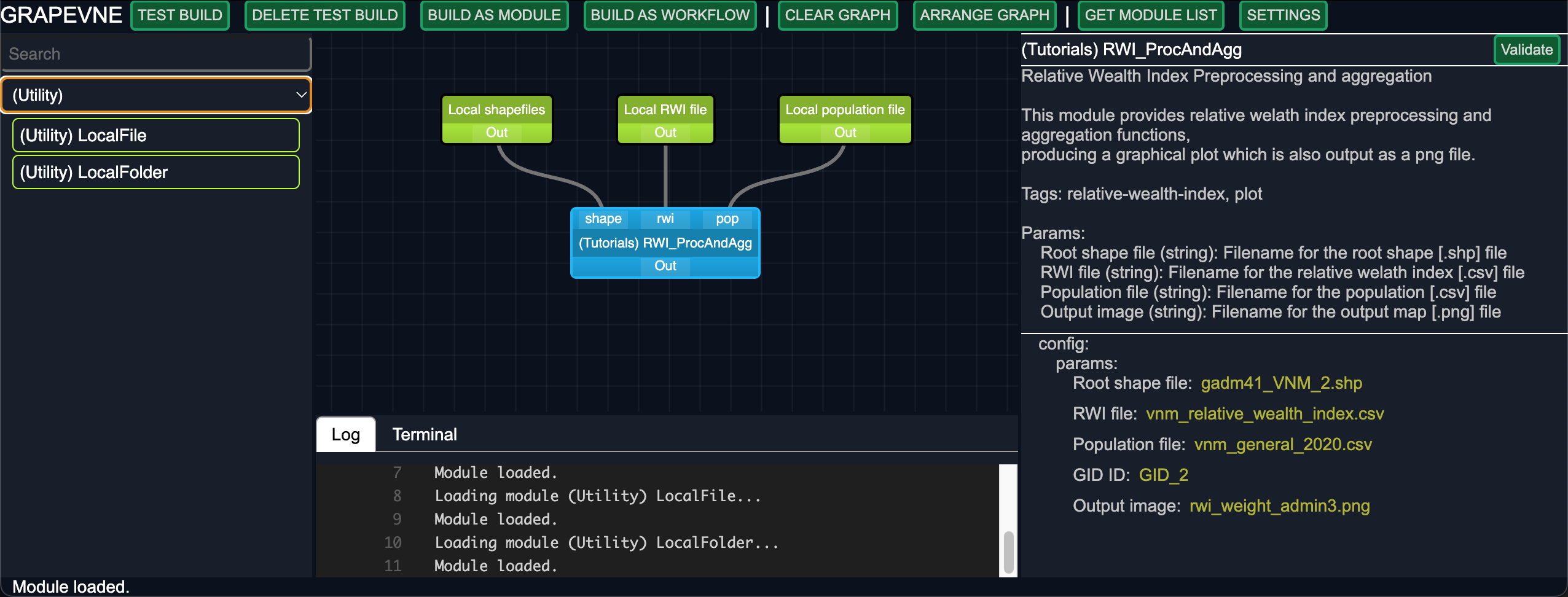
Your final workflow should look something like this:

We are now ready to Build and Test run your workflow. After waiting a minute or two for the conda environments to download, you will see a Log message stating that your conda environment has been activated. The script itself takes several minutes to run, but when it is finished you should see Workflow complete and you will have access to your analysed shapefile in the results folder.

Note

As above, you may experience an issue loading packages on newer Apple Mac computers. To resolve this issue within GRAPEVNE open the Settings pane and enter the following under Environment - variables: CONDA_SUBDIR=osx-64. You can add multiple environment variables here by separating them with semicolons.

You can switch to the build-in Terminal to open the image. On MacOS the command will be similar to: open results/tutorials_rwi_procandagg/rwi_weight_admin3.png. Congratulations, you are now equipped to convert your standalone scripts into reusable GRAPEVNE modules!

Wrapping a Script in a Module

Contents

Wrapping a Script in a Module#

Parameterisation#

Implementing command line arguments in the script#

Modularise#

config.yaml#

Snakefile#

conda.yaml#

Integration with GRAPEVNE#

Testing with snakemake#

Loading into GRAPEVNE#